Allegion Developer Portal
Allegion Developer Portal

The Schlage ENGAGE Gateway uses Bluetooth® Low Energy technology to communicate to ENGAGE enabled devices in real time. Communication is actively maintained in order to support host command/response operations as well as the continuous flow of device reported status.
Ensuring that this communication can occur with reliability can be challenging. As with all wireless technologies, the propagation of radio waves and the presence of interfering signals makes predicting results difficult without deeper planning.
This document presents recommendations and guidance for conducting a site survey when planning ENGAGE Gateway installations in order to maximize communication reliability.
Bluetooth® Low Energy (BLE) is a wireless personal area network technology aimed at low power consumption applications. Generally, the low power device is called a “peripheral” and advertises its services periodically such that other devices can detect and establish a connection if desired.
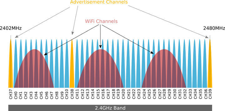
BLE makes use of the 2.4GHz ISM frequency band, dividing the spectrum into 40 equivalently spaced channels. Of the 40 available communication channels, 37 of them are reserved for linked communication with the remaining 3 reserved for advertising. Each of the channels is 1MHz wide and separated by 2MHz. It should be noted that the 2.4GHz frequency band is also shared with traditional Wi-Fi b/g/n devices. This is illustrated in Figure 1.
All wireless ENGAGE devices use BLE as the common method of communication to an ENGAGE Gateway. After linking, the ENGAGE Gateway will continuously scan for that linked device’s advertisements and establish connection. Should some interruption in connectivity occur (loss of power, high momentary RF interference, etc.), the Gateway will re-establish the connection as quickly as possible.
As the effective transmission rate over BLE is quite low and the time it takes to re-establish a connection can be on the order of 10’s of secs (typically 5-25 secs), it is essential that disconnections be minimized.
The goal of an ENGAGE wireless site survey is to determine the number and placement of Gateways that will minimize connectivity disruptions and maximize throughput to all planned ENGAGE devices.
The following are general guidelines for conducting a wireless site survey:
The datasheets and user installation manuals of ENGAGE devices detail specific placement considerations and maximum possible wireless communication ranges. These values are clear line-of-sight recorded capabilities. For the Gateway, maximum antenna range is 100ft (30.5m).
A building blueprint or other detailed depiction of the location of walls, hallways, stairwells, etc. is an important component for planning and ultimately marking where the various ENGAGE Gateways should be placed.
Walk through the facility in order to verify the accuracy of the facility diagram and make note of any and all potential RF attenuation barriers or large RF noise sources.
a. Inspect the facility – Physical Obstructions.
As a quick rule of thumb, think of RF energy as light. From a proposed placement location, if you cannot orient a flashlight such that it would be able to directly shine light onto the intended target, then clear line-of-sight cannot be established. In terms of ENGAGE Gateway placement, a conservative estimate for when clear line-of-sight cannot be achieved due to some major obstruction is to assume the maximum effective distance to the target has now been halved. Returning to the light analogy, if by moving the flashlight in a straight line beyond the impediment still would not result in direct illumination of the intended target, then again the effective distance should be halved; that is repeat this halving of distance for each major impediment encountered or for each “reflection” (think: bouncing the flashlight’s beam on a mirror) required to reach the intended target.
NOTE: RF signals cannot pass through metal or metal mesh (stucco) at all. Large metal cabinets/racks, or specialty partitions/pillars, etc. are not usually indicated on facility diagrams but can impede signals more significantly then any denoted fixed boundary. Add markers for these to the facility diagram and assume effective maximum distance goes to zero when passing through metal or metal mesh entities.
By using the above approximation method for effective maximum distance, one can begin to determine approximate number and location of Gateways needed in order to cover the furthest and most difficult to reach intended targets.
b. Inspect the facility – RF Noise
Besides physical obstructions, RF noise pollution is everywhere. Any significant digital appliance will give off some radiation. Indicate server rooms and/or large clusters of electronic equipment on the facility diagram in order to avoid placing Gateways near these sources of interference as much as possible. Likewise, placement should be avoided near electric motors and generators, microwave ovens, large RF radios, medical equipment, high-voltage ballasts of neon signs, industrial machinery, elevators, and large switching power supplies. However, the least obvious but most probable source of ambient RF interference is an existing wireless infrastructure. Enterprise level access points are likely installed throughout the facility and contain line-powered antennas that transmit at higher signal strengths than battery operated BLE devices. As such, it is important to place Gateways at least 10ft (and preferably more) from any WiFi access point. Gateway to ENGAGE edge device communication can be severely degraded due to continuous high bursts of RF interference should the WiFi access point be too close to an ENGAGE entity. Additionally, be sure to think three-dimensionally should the facility have multiple floors. RF signals will penetrate floors and ceilings and Gateway placement should consider where other Gateways and existing wireless infrastructure above and below exist or will occur; when referencing the facility diagram, consult the floors above and below for any infrastructure markings you made during the inspection and adjust proposed Gateway location configurations away from directly stacking such RF sources on top of each other.
While BLE is designed to handle transitory RF interference through frequency hopping and the Gateway will perform automatic reconnection to a linked device should interference become so great that a temporary disconnect occurs, continuous high levels of ambient RF noise will degrade overall effective communication. Using an RF spectrum analyzer, one can measure the ambient RF noise in an environment. A description of how to setup and use one such device follows this document. Additionally, as WiFi access points are generally the abundant producers of background 2.4GHz noise in a typical office or high rise facility, using a freeware WiFi scanner to survey the band can give you a quick feel to the level of RF interference in an area.
In Figure 2, the free Android mobile Application “Wifi Analyzer” by farproc, is used to assess a facility’s Wi-Fi infrastructure. The application was set to monitor the 2.4Ghz band and shows numerous access points spread across all the primary WiFi non-overlapping channels (1, 6, 11). In this busy RF environment, a peak RF noise value of -83.5dBm was measured using an RF Explorer 24G (shown in Figure 3). Again, while peak can be an interesting figure, it is actually the average RF noise value that matters more. In this case, the average RF noise value was measured at -90.3dBm, a value that will still support linked devices in the medium signal strength range satisfactorily when using the latest Gateway and linked device firmware.
| Figure 2: farproc’s WiFi Analyzer for Android Devices | Figure 3: Measuring Ambient 2.4Ghz RF noise |
|---|---|
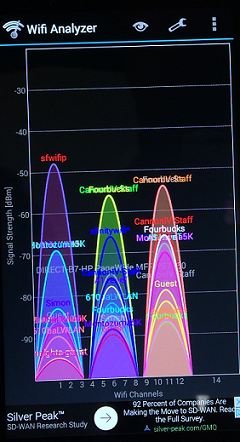 | 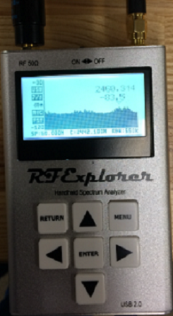 |
While touring the facility, use a 2.4GHz RF Spectrum Analyzer and indicate any high noise areas on your facility diagram. For high ambient RF noise areas, Gateways should be placed closer to their intended linked devices with clear line-of-sight to maximize signal strength. Consult the Figure 4 graph for recommendations on average noise levels to signal strengths necessary for optimal operation.
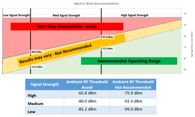
Figure 4 makes explicit the graph cutoff values for both too much noise present (Ambient RF Threshold Avoid) and not recommended configurations (Ambient RF Threshold Not Recommended). Areas with measured ambient 2.4GHz RF noise above the high signal strength’s associated Ambient RF Threshold Avoid need to be reassessed in terms of ENGAGE device placement. Ideally, noise sources can be identified and removed such that operation within the area can be better assured; otherwise, operation within such exceedingly high ambient RF noise environments is likely impractical and any such configuration should be monitored continuously after deployment for real-world reliability.
Additionally, while low signal strength cutoff values are shown in the table for completeness, just as one would not expect good results using a cellular phone with only one bar of reception, final configurations that result in linked devices having low signal strengths at the Gateway should also be avoided.
From the initial assessments made during Step 3 Inspect the Facility, one should have a good idea of where Gateways will be needed, approximately where to place them, and the target signal strengths to achieve in potentially problematic areas. Through the use of a BLE scanner and an ENGAGE lock on a desktop mount, one can refine this potential Gateway location for performance needs.
This assessment intends to optimize placement of a Gateway by finding a location that ensures strong RF signal strengths across all intended devices for link.
Place the mounted lock at the base of the target portal (doorway), turn the inside lever of the lock to ensure it is advertising, and then move to the proposed location for the associated Gateway.
Using a freeware Android BLE scanner application (suggestions are BLE Scanner by Bluepixel Technologies or Bluetooth 4.0 Scanner by John Abraham), perform a Bluetooth Low Energy scan of the area and find the lock in the scan list by using the name assigned to the lock during commissioning. You may need to stop the scanner if lots of BLE devices are present in order to search the list for the particular lock in question. Some scanners show the lock names (e.g. AQ Conference) as part of the description field (Figure 5) and others display the advertising name directly (Figure 6).
| Figure 5: Bluetooth 4.0 Scanner by John Abraham for Android Devices | Figure 6: BLE Scanner by Bluepixel Technologies for Android Devices |
|---|---|
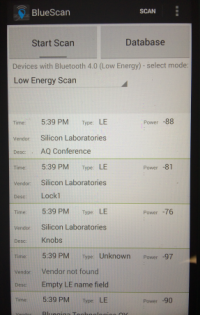 | 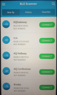 |
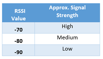
Stop the scan and record the RSSI value (sometimes called power) displayed by the scanner for the lock at the proposed Gateway location. Without moving, run and then stop the scan again, to obtain a second RSSI value. Finally, repeat the run/stop scan operation for a third value. The median (or middle) value will be the one used for the exercise. The chart below gives approximate signal strengths one will likely see for RSSI median values at or above the indicated number.
NOTE: All devices have different antennas and that even depending on how you hold the mobile device you could introduce attenuation as well. The goal here is not to verify any exact value but rather that a reasonable signal strength is being achieved to the target ENGAGE device from the proposed Gateway location. Aim for an approximate signal strength of medium or better, adjusting your proposed Gateway location accordingly to achieve it. Remember though that if high ambient RF noise is present, higher signal strengths are necessary as well.
Move the mounted lock to another portal location intended to be served by the same Gateway. Repeat the process of turning the inside level, moving back to the proposed Gateway location, and performing the three RSSI value scans to obtain first a median RSSI and then an approximate signal strength associated with that portal.
Repeat the operation of obtaining an approximate signal strength to each portal intended to be connected to the Gateway at that location and then verify that these approximate strengths meet your performance and ambient RF noise needs.
Figure 8 shows various large scale transfers from a Gateway to a linked device. In general, large scale transfers only occur in IP mode for databases containing many users or during firmware update operations. For comparison, an NDE firmware image is about the same size as a ‘minified’ (all white-space removed) 5000 user database (~1MB). The Gateway has a maximum transfer rate to a device over BLE of 768 bytes/sec. Using the 5000 user database as an example then, the best case transfer time is ~22 minutes, with typical real-world office environment transfer times measured at ~50 minutes. It should be noted that with latest Gateway and lock firmwares, even low signal strength transfers of large files completed successfully. Duration of transfer increases, however, as signal quality (strength/noise) degrades and the number of disconnections and retries goes up as a result.
![]()
For completeness, the following are the characteristics of the testing shown in Figure 8.
| Test Setup (an ambient RF noise of -90.3dBm measured for all test cases) | Signal Strength Reported at GW to lock | Effective Rate (linear trend) |
|---|---|---|
| NDE and GW \~8ft apart no obstructions | High | \~10.3min / 1000 users |
| NDE and GW \~45ft apart Thru two standard office walls | Medium | \~11.9min / 1000 users |
| NDE and GW \~45ft apart Thru two standard office walls and one set of large metal cabinets | Low | \~19.6min / 1000 users |
Once satisfied with the proposed Gateway location maximizing approximate signal `` strength and in accordance with ambient RF noise considerations, it is time to test a real configuration. The mounted ENGAGE lock should now be commissioned to a Gateway.
For this exercise, perform the following steps:
1. Perform standard Gateway commissioning followed by a standard lock linking operation
for the mounted lock using the ENGAGE mobile application before proceeding. Consult the
Gateway Installation Instructions and User Guide for more details.

2. Place the mounted lock at the base of the target portal (doorway) and then move to the
proposed location for the associated Gateway. For efficiency, multiple mounted locks – one
placed at each of the target portals to be linked to the Gateway in this vicinity - can be
used to conduct the exercise with simultaneous results available.

3. Temporarily hold or mount the Gateway at the proposed location, providing power to the device.

4. Once the Gateway is fully operational (solid blue), connect to the Gateway using the ENGAGE
mobile application. Once connected, select “Manage Linked Devices” to display all linked locks
to the Gateway and their associated signal strength. Figure 9 shows the three possible signal
strength indications the Gateway can indicate for a linked device.
Figure 9 – Gateway Reported Signal Strengths to a Linked Device (High, Medium, Low in order shown)**
5. Ensure that the reported signal strength is up to date and correct by pulling down on the
screen to force a refresh. Wait 5 minutes and repeat the refresh to verify the signal strength
reported remains as reported before.

6. Confirm that the reported signal strength is in-line with expectations based upon your prior
wireless site survey exercises and that the signal strength will be adequate for the area’s
measured ambient RF noise (Figure 4).

7. If the signal strength is not in-line with expectations, re-perform the tasks: **Refine
Preliminary Gateway Locations** and **Validate Final Gateway Locations** to ensure placement
and then adjust the Gateway in small (\~2ft) increments across each axis in turn until a better
position is determined.

8. If not conducted simultaneously for all portals, repeat the above process for each portal that
will contain a linked device to the Gateway.

    **NOTE:** If significant adjustment of the Gateway becomes necessary due to a subsequent portal’s
verification, then all previous portals should be revisited in light of the new proposed placement.
It is for this reason that multiple mounted locks pre-linked to the Gateway is again suggested to be
used for performing validation of all linked devices’ signal strengths simultaneously rather than
individually.

9. Once the ultimate location for the Gateway has been confirmed, update your facility diagram clearly
indicating the final exact placement location and proceed to formal installation of the Gateway.
When conducted properly, a wireless site survey can help ensure that ENGAGE BLE communication will occur reliably and efficiently. While the steps presented in this document may be tedious, for complex facilities with challenging RF environments, they can prove vital to isolating problem areas and determining proper mitigations in the form of additional Gateway needs or non-obvious modifications to placements.
The RF Explorer 24G is a handheld spectrum analyzer which can be utilized to measure the amount of ambient RF noise in the surrounding atmosphere. This can be helpful to analyze how much interference or resistance to communication may be present in low power RF devices.
Bluetooth Low Energy utilizes the 2.4 GHz ISM frequency band which is subdivided into 40 equivalently spaced channels. Each of the channels is 1MHz wide and separated by 2MHz.
Figure A-1 shows a typical 2.4GHz frequency analysis of the ambient RF noise. The down arrow is illustrating that the current average peak frequency is at 2413.142MHz with a level of -85dBm. It can be seen from this measurement that the overall average ambient noise is less than -85dBm with a small peak towards the lower end of the frequency spectrum.
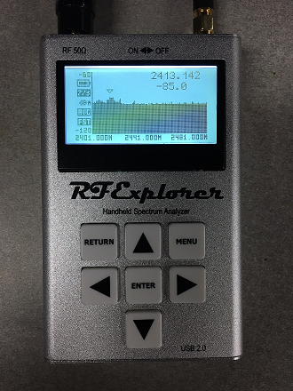
The following sections describe how to configure the RF Explorer to take RF noise readings as shown in Figure A-1. Note that the top range (dBm) of the shown plot can be modified by clicking the up and down arrows to allow for ease of viewing and increased resolution with different noise levels.
Once the RF Explorer is turned on, the default plot should be displayed automatically.
To navigate into the menu, please use the MENU button. The MENU button is also used to move from one menu to the next.
The left and right arrows can be used to move from one menu to the next when a menu option has not been selected. Once a menu option has been selected the left and right arrows are used to choose different selections in that specific menu option.
Once the appropriate menu screen is displayed, the up and down arrow keys are used to select the appropriate setting. Once a menu option has been selected the up and down arrows are used to choose different selections in that specific menu option.
Once the appropriate setting is highlighted, the ENTER key is used to select that option and allow for modifications if allowed.
The return key is used to return to the previous screen or the plot, whichever is applicable. The menu can be re-entered by pressing the MENU button after the RETURN button has been pressed.
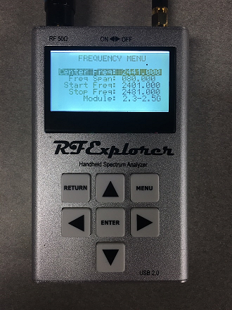
There are three main menus which need to be configured consisting of the Frequency, Attenuator, and Configuration menus. Each of these menus is described in detail below.
These settings allow you to configure the frequency span of the graph:
Center Frequency: 2441.0000
Frequency Span: 080.000
Start Freq: 2401.000
Stop Freq: 2481.000
Module: 2.3-2.5G
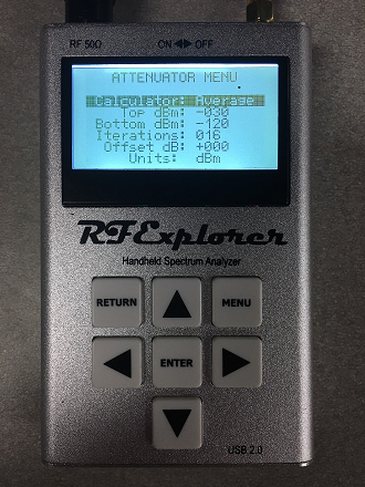
These settings allow you to configure the decibel range of the graph:
Calculator: Average
Top dBm: -030
Bottom dBm: -120
Iterations: 016
Offset dB: +000
Units: dBm
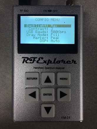
These settings allow you to set the configuration of the graph:
Backlight: Max
Contrast: 3
USB Bauds: 500kbps
Draw Mode: Fill
Marker: Peak
DSP: Auto
.png)